Efficiently estimating the trace \(\textrm{tr}(A) = \sum_{i=1}^d A_{ii}\) of a square matrix \(A \in \mathbb{R}^{d \times d}\) is an important problem required in a number of recent deep learning and machine learning models. In those cases the matrix \(A\) is typically positive-definite, large and dense.

As a sample of recent occurences of needing to compute the trace of large matrices in machine learning, I picked the following applications.

• Continuous normalizing flows, as in diffusion models (Song et al., ICLR 2021), FFJORD (Grathwohl et al., ICLR 2019) and Neural ODEs (Chen et al., NeurIPS 2018), where an initial sample \(x(0) \sim p_0\) is continuously transformed by a function, i.e. \(\partial x(t)/\partial t = f(x(t),t)\) from \(t=0\) to \(t=1\). To evaluate \(\log p(x(1))\) we need to rely on the instantaneous change of variable formula,
  $$\frac{\partial \log p(x(t))}{\partial t} = -\textrm{tr}\left( \frac{\partial f}{\partial x(t)}\right),$$
  such that the log-probability is determined by
  $$\log p(x(1)) = \log p(x(0)) - \int_0^1 \textrm{tr}\left( \frac{\partial f}{\partial x(t)}\right)\,\textrm{d}t.$$
  Computing the trace of the Jacobian \(\frac{\partial f}{\partial x(t)}\) is the computational bottleneck.
• Efficient Gaussian Process evidence computation. (Wenger et al., ICML 2022), where trace estimation is used to estimate the log-marginal likelihood, and the matrix \(A\) is a kernel matrix.
• Approximating log-determinants in invertible ResNets. (Behrmann et al., 2018) propose a variant of ResNet blocks that is invertible by constraining the Lipschitz-constant of the ResNet block update to be smaller than one. Once invertible the ResNet block can be used for generative modelling via a normalizing flow model. That is, we sample \(x_0 \sim p_0\) from a simple prior \(p_0\) and then map \(f(x_0)\) to the target density. To compute log-likelihoods for a given \(x\) we invert the map and compute \(\log p(x) = \log p_0(f^{-1}(x)) + \log |\det J_{f^{-1}}(x)|\). By exploiting the structure of the \(i\)'th ResNet block, \(f_i(x) = x + g_i(x)\), and the Lipschitz constraint on \(g_i\), the log-determinant computation can be reduced to a convergent power series, \(\textrm{tr}(\log (I + J_g(x))) = \sum_{k=1}^{\infty} \frac{(-1)^{k+1}}{k} \textrm{tr}(J^k_g).\) Without going into detail, Behrmann et al. truncate the power series and compute the trace terms using Hutchinson's trace estimator, thus are able to use invertible ResNets for generative modelling. The same group, in (Chen et al., 2019), improve on the finite truncation by using stochastic truncation in the form of Russian roulette estimators, managing to create unbiased estimates, again using trace estimation for each term of the power series. (If you hear the term "Russian roulette estimator" for the first time, it is a quite general technique that is worth knowing about; a good self-contained brief introduction and history of randomized series truncation can be found in section 2.1 and 2.2 of (Beatson and Adams, 2019).)
• Regularizing continuous dynamics. (Finlay et al., ICML 2020) regularize the Frobenius norm \(\|A\|_F^2 = \textrm{tr}(A^T A)\) of the Jacobian of a neural ODE leading to smoother dynamics and fewer adaptive integrator steps.
• Neural network quantization layer-wise sensitivity metric. (Dong et al., NeurIPS 2020) and (Qian et al., 2020) use the trace-of-Hessian of parameters belonging to the same neural network layer to allocate the quantization fidelity needed. Such a trace-of-Hessian regularization is also effectively used in one of the early papers on energy-based models, (Kingma and Le Cun, 2010), there it is used to regularize the curvature of learned energy functions. The diagonal of the Hessian is a natural local sensitivity measure and perhaps the earliest use in neural networks is in the classic optimal brain damage sensitivity metric of (Le Cun et al., 1989), which used second derivatives for each parameter to determine deletion of neurons.
• Sliced score matching. (Hyvarinen, JMLR 2005) introduced score matching as a learning objective for energy-based models, \(p(x) \propto \exp(-E(x))\), and in the score matching objective a sum of second derivates of the energy function needs to be evaluated, \(\sum_{i=1}^d \partial^2 E(x) / (\partial x_i)^2\). Because evaluating these second-order derivates is expensive this limited the applicability of score matching until (Song et al., UAI 2020) introduced sliced score matching where the expensive term is replaced by a stochastic estimate \(\mathbb{E}_z\left[\sum_{i=1}^d \sum_{j=1}^d \frac{\partial^2 E(x)}{\partial x_i \, \partial x_j} z_i z_j\right]\), i.e. a Hutchinson estimate of the trace of the Hessian of \(E\). For a great overview of these techniques see the recent review by (Song and Kingma, 2021).

What is the shared difficulty in all of the above applications? After all, computing the trace of an explicitly given matrix \(A\) is trivial: simply sum the diagonal elements,

However, in the above applications arising in deep learning the problem is that it is very expensive to compute \(A\) explicitly, but we can query matrix-vector products efficiently. Given \(z \in \mathbb{R}^d\), we can efficiently compute

Clearly, if we are able to compute many such products, say \(d\) times, we can reconstruct the matrix \(A\) completely. The simplest example is to take \(z^{(m)} := e_m\), the natural basis vectors in \(\mathbb{R}^d\), such that \(y^{(m)} = A \, z^{(m)}\) directly extracts the \(m\)'th row of the matrix. By extracting all rows we could obtain \(A\) in explicit forms.

The drawback of this technique is that performing many matrix-vector multiplications is expensive, where typically each matrix-vector product corresponds to one forward-backprop operation in a neural network. Is there a better way, requiring only a small number of matrix-vector products to obtain an accurate estimate of the trace of \(A\)?

Yes, and we will discuss the main technique below. But first, to add more excitement to our goal: if the problem of trace estimation is amenable, a number of related problems are also in reach using extended methods such as variants of conjugate gradients (Seeger, 2000) and the stochastic Lanczos quadrature method of (Ubaru et al., 2017) which allows efficient estimation of functions of the form

where \(f: \mathbb{R} \to \mathbb{R}\) is a scalar function and \(\textrm{tr}(f(\cdot))\) is the resulting trace function, \(\textrm{tr}(f(A)) := \sum_{i=1}^d f(\lambda_i(A))\). Through different choices of \(f\) trace functions enable estimation of other quantities,

• Log-determinants, \(\log \det(A) = \textrm{tr}(\log(A)) = \sum_{i=1}^d \log(\lambda_i)\).
• Nuclear norm, for \(X \in \mathbb{R}^{k \times d}\) defined as \(\|X\|_* = \textrm{tr}(\sqrt{X^T X})\), and more general Schatten \(p\)-norms.
• Trace of \(A^{-1}\), where \(\textrm{tr}(A^{-1}) = \textrm{tr}(f(A))\) with \(f(t)=1/t\).

As we will see below, another quantity that can be estimated using Hutchinson-style estimators is the diagonal of a matrix \(A\).

Skilling-Hutchinson 1989 trace estimator

The estimator appeared in two works in parallel. In his original 1989 paper, (Hutchinson, "A Stochastic Estimator of the Trace of the Influence Matrix for Laplacian Smoothing Splines", 1989), Hutchinson introduced the first stochastic estimator of the matrix trace, and simultaneously John Skilling introduced the same technique in (Skilling, "The Eigenvalues of Mega-dimensional Matrices", 1989).

The Skilling-Hutchinson trace estimator is not just historially interesting; it is still the most common method used today due to its general applicability and simplicity of implementation.

Skilling-Hutchinson's trace estimate: If \(z \in \mathbb{R}^{d}\) is a random vector satisfying \(\mathbb{E}[z z^T] = I\), then

The Skilling-Hutchinson estimator is

where \(z^{(m)}\) are random vectors satisfying the above condition. In Hutchinson's original estimator these vectors are Rademacher vectors with elements iid in \(\{-1,1\}\) and we write \(\hat{T}_{H,M}\), but the term Hutchinson's trace estimator is also commonly used nowadays if standard Normal vectors are used in the Gaussian trace estimator \(\hat{T}_{G,M}\).

The Skilling-Hutchinson estimator is unbiased, meaning \(\mathbb{E}[\hat{T}_{\cdot,M}(A)] = \textrm{tr}(A)\). Moreover, it is known that for standard Normal vectors we have

where \(\lambda_i(A)\) is the \(i\)'th Eigenvalue of \(A\). For Rademacher vectors it is known that

You can see that using Rademacher vectors has provably smaller variance than using Gaussian vectors,

There is a wealth of theory available for the estimator, and a good recent entry point into known results is Maciej Skorksi's paper "A Modern Analysis of Hutchinson's Trace Estimator" from 2020 (PDF). In it he gives a error bound for the Rademacher version, using the relative error

For this error and for any \(d \geq 2\) he gives the tail bound for any \(0 < \varepsilon < 3/8\) of the form

Praise for Hutchinson's estimator

There is a lot of good to say about Hutchinson's trace estimator:

It is simple: the estimator is easy to understand and implement. It is free from exotic ingredients, uses just basic linear algebra, and does not make strong assumptions thus is widely applicable. Because it is simple it works well with auto-differentiation.

Linear trade-off \(M\): Hutchinson's estimator comes with a free choice of \(M \geq 1\), the number of matrix-vector products to evaluate. The parameter \(M\) linearly controls both variance and computational effort with the estimator becoming exact for \(M \to \infty\).

Parallelizable: for larger values of \(M\) all evaluations can be done in parallel, i.e. the sequential compute depth does not increase for more accurate estimates.

Unbiasedness: for any \(M \geq 1\) the estimator is unbiased. How valuable is an unbiased estimator? In general whether an estimator is unbiased or not may not matter (see Andrew Gelman's points here and here). But our situation here is special for two reasons: 1. there is an exact quantity of interest, \(\textrm{tr}(A)\), and our estimation is done only for computational benefits; and 2. for most deep learning applications it is incredibly important: it allows iterative stochastic optimization algorithms to work correctly and to asymptotically average out estimator variance.

So is all good then with Hutchinson's estimator?

Problems of Hutchinson's estimator

Despite singing the praise just now, the estimator has a number of fundamental problems as well.

High Monte Carlo variance: the estimator has a decaying variance at rate \(O(1/M)\) arising from taking the average of \(M\) estimates. To see why this is a bad rate, consider the case where we take \(M=d\), and we take Normal vectors \(z^{(m)} \sim \mathcal{N}_d(0,I)\). We then could recover the exact matrix \(A\) and thus its trace without any uncertainty. Hutchinson would still offer us only a \(1/d\) decrease in variance and hence does not use all information contained in our measurements.

The analysis from Skorski reflects this hungryness for large sample sizes. Skorksi's analysis estimates that for given \((\varepsilon,\delta)\) parameters, we need \(n(\varepsilon,\delta) = 2(1-(8/3)\varepsilon)\log(1/\delta)/\varepsilon^2\) samples to achieve an absolute bound of \(\varepsilon\) on the relative error with probability \(1-\delta\). As an example, his results requires that \(n(0.1, 0.1) = 337\) and \(n(0.01, 0.1)=44824\) for example, independent of \(d\).

Complete prior ignorance: in some applications we may have a prior idea about \(A\) or of its trace value. For example, in deep learning we learn iteratively by gradient descent, and a matrix \(A_t\) at step \(t\) may not be too different from a matrix \(A_{t+\Delta}\) for small \(\Delta\).

Complete random design \((z^{(1)},\dots,z^{(M)})\): whether Normal or Rademacher vectors are used, the random vectors \(z^{(m)}\) are chosen independently at random. Can we improve the estimate by chosing them dependently? Or by chosing \(z^{(m)}\) adaptively based on \((y^{(j)},z^{(j)})_{j < m}\)? The latter is an adaptive experimental design and may or may not be an option depending on our needs to parallelize computation over \(z^{(m)}\)'s.

Variance Reduction Approaches

A number of approaches have been proposed to preserve the spirit of the Hutchinson estimator but to lower its variance. The shared idea is to think sequentially and to use prior measurements to construct some form of estimate \(\hat{A}\) of \(A\), which can then be used to lower the variance.

I am aware of two classes of methods: one based on control-variates, and one based on constructing a low-rank approximation to \(A\).

In addition to these two classes, I will also throw in an attractive new method into the mix, based on randomized quasi Monte Carlo.

Control-variate Methods

Control variates are a classic method for variance reduction and are frequently used in reinforcement learning, where they are called baselines. A great introduction to classic variance reduction methods can be found in Chapter 8 of Art Owen's yet-unreleased Monte Carlo book, with Section 8.9 introducing various forms of control variates.

In its simplest form the idea is this: we are interested in estimating \(\mathbb{E}_{z \sim p}[f(z)]\) using samples from \(p(z)\). If we know a "simple" function \(h\) and this function is similar to \(f\), i.e. we have \(h(z) \approx f(z)\), then we can instead attempt to estimate the equivalent quantity

The first expectation is now likely smaller in magnitude, so our Monte Carlo estimate of this first term has smaller variance. But what about the second term? If \(h\) is simple enough we may be able to compute this quantity analytically, with no Monte Carlo variance at all.

To make this idea realistic, we typically relax the definition somewhat and define \(h_{\beta}(z) := \beta \, h(z)\), where \(\beta \in \mathbb{R}\) can be estimated to maximally mimic the behaviour of \(f(z)\) and thus to reduce the variance of \(f(z) - h_{\beta}(z)\) the most.

For trace estimation (Adams et al., 2018) first proposed to use control variates to reduce variance:

• They propose to set \(h_{\beta}(z) = \beta \, z^T B z\), where \(B \in \mathbb{R}^{d \times d}\) is a matrix chosen by us, ideally \(B \approx A\), and \(\beta \in \mathbb{R}\) is estimated or fixed to \(\beta=1\).
• The \(M\)-sample trace estimator now becomes
  $$\hat{T}_{C}(A,B,\beta) = \frac{1}{M}\sum_{m=1}^M \left[(z^{(m)})^T A z^{(m)} - \beta (z^{m})^T B z^{(m)}\right] + \beta \textrm{tr}(B).$$
• When \(z^{(m)} \sim \mathcal{N}_d(0,I)\), Adams et al. show (Lemma 4.1 in their work) that the variance-minimizing choice of \(\beta\) is \(\beta^* = \textrm{tr}(A\,B)/\textrm{tr}(B\,B)\) and that for this choice the variance of the estimator is reduced compared to the Gaussian trace estimator by \(2 \textrm{tr}(A \,B)^2 / \textrm{tr}(B \, B)\). This also shows that when \(B=A\) the estimator variance is zero.

How to select the matrix \(B\)? Adams et al. make one efficient proposal, which is to estimate the diagonal of \(A\) in the form \(B = \textrm{diag}(b)\), where \(b \in \mathbb{R}^d\). The diagonal is a simple choice because we can evaluate \(\textrm{tr}(B) = \sum_{i=1}^d b_i\) but also because the Hutchinson-style trace estimator already contains an estimator of the diagonal within it:

where \(\odot\) is the elementwise product. This identity holds for both the Rademacher vectors and the Gaussian vectors because \(\mathbb{E}[z_i^2] = 1\). For the \(i\)'th element of the diagonal, we can see that

Adams et al. also propose to apply the control variate idea once more to the diagonal estimate itself. To see one way to achieve this is to look at the \(m\)'th iteration, where our instantaneous diagonal estimate is

Instead we can use our existing knowledge of \(A\), in the form of \(\hat{b}^{(m)}\):

Putting the two control variate ideas together, we can implement the Adams et al. trace estimator in the following Julia code.

function adams_trace_estimator(A, M::Int; use_diag_cv=false)
    d = size(A,1)
    b_diag = zeros(d)   # B = diag(b_diag)

    tr_est = 0.0
    for m = 1:M
    z = randn(d)    # Gaussian z^{(m)}
    y = A*z

    y_B = b_diag .* z   # B z
    tr_est += z'*y - (z'*y_B - sum(b_diag))   # z'Az - (z'Bz - tr(B))

    # Update diagonal estimate
    if use_diag_cv
        b_diag_cur = (z .* (y - y_B)) + b_diag  # z .* ((A-B)z) + diag(B)
    else
        b_diag_cur = z .* y   # instantaneous estimate of diag(A)
    end
    b_diag .*= (m-1)
    b_diag += b_diag_cur
    b_diag ./= m        # Invariant: b^{(M)} = (1/M) sum_{m=1}^M (z^{(m)} .* y^{(m)})
    end
    tr_est / M, b_diag
end

Low-rank Approximation Methods (Hutch++)

(Meyer et al., 2021) present improvements on the Hutchinson estimator by first extracting a low-rank approximation to \(A\) and then using this low-rank approximation to reduce the variance of the trace estimate.

Given a good approximation \(\tilde{A}\) of \(A\) the method also uses the same technique as the control variate approach, representing

where \(\textrm{tr}(\tilde{A})\) is computed analytically and the second term is stochastically estimated at reduced variance. How to obtain a good approximation \(\tilde{A}\)? Meyer et al. make two proposals, which then form the Hutch++ and the Nystroem-Hutch++ estimator. I will only discuss the Hutch++ briefly here.

Hutch++ estimator. Given a symmetric psd matrix \(A \in \mathbb{R}^{d \times d}\) and an overall budget of \(m\) query vectors, split this budget into \(q_k\) and \(\ell\) such that \(2 q_k + \ell = m\). Create \(S \in \mathbb{R}^{d,q_k}\) with each element \(S_{ij} \sim \mathcal{N}(0,1)\). Evaluate \(Y = A S\) and orthonormalize \(Y\) to \(Q \in \mathbb{R}^{d \times q_k}\). Set \(\tilde{A} = Q^T A Q\) and apply the control variate method on \(\ell\) additional samples.

In Julia this can be implemented as follows.

function hutchpp(A,m)
    d = size(A,1)
    k = floor(Int, (m-2)/8)   # Variance-optimal allocation of initial queries
    qk = 2*k+1                # qk: number of initial query vectors
    ell = m - 2*qk            # ell: remaining budget for final estimate
    @assert (2*(qk)+ell) <= m # make sure total query budget m is satisfied

    # initial basis construction
    S = randn(d, qk)      # qk initial query vectors
    Y = A*S              # query matrix
    Q = Matrix(qr(Y).Q)  # orthonormalize SY to a (d,qk) basis

    # variance-reduced stochastic estimate
    z = randn(d,ell)      # ell remaining queries
    y0 = A*z
    y = y0 - Q*(Q'*y0)    # adjust estimate using low-rank approximation
    tr_ests = sum(z .* y, dims=1)
    tr_est = Statistics.mean(tr_ests) + tr(Q'*A*Q)   # another qk queries
    tr_est
end

A problem of the Hutch++ family of estimators shared with the control variate one is that it is difficult to parallelize: there are two sequential steps and the second step relies on the output of the first. This may not be a problem in most applications, but in training deep neural networks we typically prefer parallelization.

Preconditioning

If the matrix \(A\) is a kernel matrix, i.e. \(K_{ij} = k(x_i, x_j)\) for some kernel function \(k\), then variance of a stochastic trace estimator can be greatly reduced using an appropriate preconditioner.

An extensive set of results is given by (Wenger et al., "Preconditioning for Scalable GP Hyperparameter Optimization", ICML 2022) with the application of computing the log-marginal likelihood (evidence) of Gaussian processes.

In their application, they exploit the identity

and estimate the second term using a stochastic trace estimator for variance reduction.

Wenger et al. show in theory and through experiments that this leads to large reduction in variance. As an example, if \(A\) is a kernel matrix arising from a radial basis function (RBF) kernel in one dimension then the variance scaling that can be achieved with a suitable precondition can be exponential, \(\mathbb{V}[\hat{T}_P] = exp(-c m)\).

The paper by Wenger et al. is very well written and the code is already available in GPyTorch.

Randomized Quasi Monte-Carlo (RQMC)

Quasi Monte Carlo methods (QMC) aim to improve on Monte Carlo integration. Whereas basic Monte Carlo methods draw samples independently, quasi Monte Carlo methods draw samples from a dependent distribution chosen such that for classes of integrands better convergence rates are obtained. Typically QMC methods start with a uniform distribution in the hypercube \([0,1]^d\). We can map the hypercube \([0,1]^d\) to a domain such as \([-\infty,\infty]^d\) using the inverse cumulative distribution function (inverse CDF) of a chosen distribution. For example, for the standard Normal distribution the inverse CDF would be the Normal quantile function. QMC points are deterministic and this determinism would lead to unavoidable bias when used for sampling. An effective remedy is to randomize QMC methods once more, by shifting all generated points using a randomly chosen offset. This is the RQMC constructions and it guarantees that the marginal distribution of every point is following the target distribution.

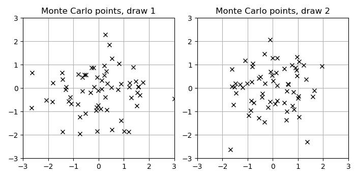
To see intuitively how selecting dependent samples could lead to better properties, here is a visual example of 64 multivariate Normal samples in 2D as used in Monte Carlo methods such as the Gaussian trace estimator:

Now, for comparison, the following Figure shows a draw of marginally Normal-distributed points generated with a RQMC construction, implemented by the following Julia code using the Sobol.jl package.

M = 64
d = 2
points = zeros(M, d)
sobolseq = skip(SobolSeq(d), max_M)
for m = 1:max_M
    points[m,:] = Sobol.next!(sobolseq)
end
points = mod.(points .+ rand(1,d), 1.0)
points = quantile.(Normal(), points)

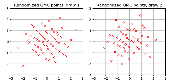
As you can see the points are more equally spaced out. The hope with RQMC methods is that such more homogeneous spacing improves the rate of the Monte Carlo average.

Formally, the starting point of RQMC methods is to assume an integration problem over a function \(f: [0,1]^d \to \mathbb{R}\). Here, for the purpose of trace estimation, we can define our function as

where \(\Psi^{-1}\) is the standard Normal quantile function, applied elementwise. We have

This construction is beneficial if we can approximate the integral of \(f\) over the \(d\)-dimensional unit cube effectively. This is what randomized QMC methods do. The theory of most QMC results requires \(f\) to satisfy bounded variation conditions on partial derivatives ("bounded variation in the sense of Hardy and Krause", aka BVHK), but these conditions can be difficult to verify. Here \(f\) has unbounded derivatives and even \(\Psi^{-1}\) itself is unbounded when approaching the boundary at zero or one. Nevertheless, we can still go ahead and simply apply RQMC methods to assess their performance empirically. This is popular practice in quantitative finance and other applications of RQMC methods, and as safety net RQMC methods typically never perform worse than plain Monte Carlo and has also been used successfully in other applications in machine learning, e.g. for variational inference in (Buchholz et al., 2018).

RQMC trace estimator. The proposed trace estimator is simply the Hutchinson construction but using a RQMC point set instead of independent samples. Here I use a Sobol sequence.

Comparison

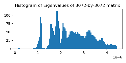
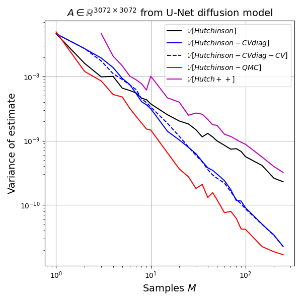
For testing the estimators we will use a matrix extracted from a recent diffusion model for image generation. This model generates 32x32x3 ImageNet images and in order to compute the training objective we need to estimate the trace of a 3072-by-3072 matrix. I extracted this implicit matrix by performing 3072 matrix-vector products with the canonical basis vectors. The matrix is quite benign, is positive-definite and has a rather smooth spectrum (see plot below). I assume these nice properties are present in most image diffusion models.

I ran 500 replicates of the following experiment: draw \(z^{(m)} \sim \mathcal{N}_d(0,I)\), \(m=1,2,\dots,250\), and pass this vector to all estimators. I record the estimate after each value of \(m\) for each replicate. Then I estimate the variance of the estimator, as well as its bias. All estimators are unbiased for all values of \(m\), as expected, so the main quantity of interest is the variance as a function of \(m\).

We can understand the variance behaviour best in a log-log plot because relationships of the form \(y=b x^{\alpha}\) become linear in the log-log plot, \(\log y = \log b + \alpha \log x\), and if the behaviour is well modelled as a line in the log-log plot, then the slope coefficient \(\alpha\) gives us the scaling behavior as \(M \to \infty\). For example, simple Monte Carlo estimates have variance behavior \(M^{-1}\) so \(\alpha = -1\). Any value smaller than \(-1\) denotes an improvement over simple Monte Carlo. Randomized Quasi Monte Carlo methods can achieve \(\alpha = -2\) for example, (Gerber and Chopin, 2015).

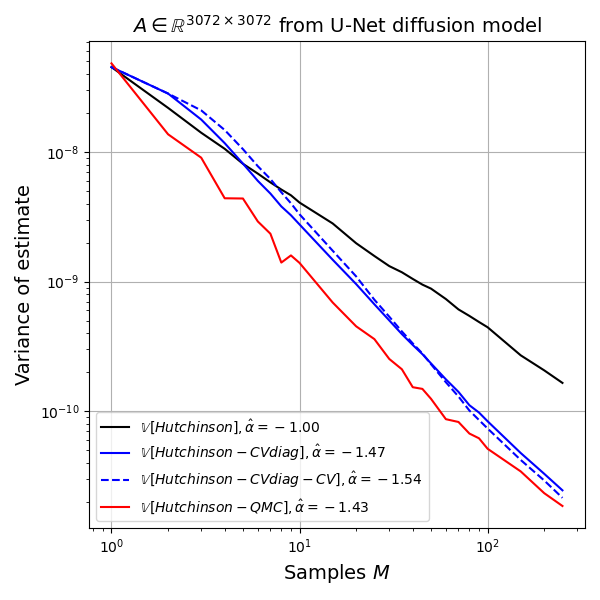
Hutch++ estimator: Unfortunately, despite solid theory in the paper, I have not been able to observe practical improvements over even the simple Gaussian trace estimate on my test matrix.

Bayesian Estimation

A classic method for approaching estimation problems is Bayesian decision theory. (Sidenote: I have mentioned (Parmigiani and Inoue, "Decision Theory: Principles and Approaches", 2009) in my blog before, but it really is a wonderful introduction to the topic.)

The key steps in the Bayesian approach are: 1. write down what you know; 2. write down how what you know relates to what you would like to know; and 3. make optimal decisions by optimizing expected utility. This recipe is simple and elegant in principle but becomes challenging quickly, as we will see shortly for trace estimation.

Benefits and Pitfalls of Bayesian Estimation

Before we look at trace estimation, I want to give one concrete example of the risks but also benefits of the Bayesian approach to estimation. This is the example of estimating the entropy of a discrete random variable discussed on this blog before. A short summary is this: between 1993-1995 David Wolpert and David Wolf proposed a sound Bayesian approach to the problem, using a standard Dirichlet-Multinomial model, which allows for efficient estimation due to conjugacy. The model appears elegant, and has support everywhere, thus can recover the true entropy and is asymptotically unbiased as well.

However, six years later, in 2001, Ilya Nemenman and colleagues found grave flaws in this benign looking Bayesian approach: the prior almost completely specifies the entropy, i.e. the prior predictive is highly concentrated when samples from the Dirichlet distribution, i.e. probability vectors, are mapped to their entropy. The full story is in my prior blog article.

It is really nice that the story does not end here: (Nemenman, Shafee, and Bialek, "Entropy and inference, revisited", 2001) proposed to add one more hyperprior layer to the Dirichlet-Multinomial model and chose this hyperprior to be maximially uninformative with respect to entropy, akin to a reference prior approach, but targetted to entropy inference. This estimator, the NSB estimator of entropy is still state-of-the-art for estimating the entropy of discrete random variables, dominating almost all other methods in terms of RMSE and bias in a wide variety of practical distribution types. However, it is computationally expensive compared to most other entropy estimates.

This story is very concrete but the lessons implied are general:

• Bayesian estimation relies on a suitable prior, and whether a prior is suitable or not also depends on the implied prior predictive over the quantity of interest.
• It may be hard to construct suitable uninformative priors, and it may not be obvious when to call a model a success.
• When a suitable prior can be designed, the Bayesian approach uses all information in the data, and can provide accurate estimates with uncertainty quantification.
• There may be a tradeoff between computational efficiency and suitability of the model.

Bayesian Trace Estimation

For Bayesian trace estimation we can propose the following directed graphical model.

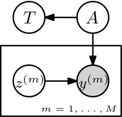
The unknown matrix \(A\) is assumed to come from a prior \(p(A)\) and \(T=\textrm{tr}(A)\) is the implied distribution over the trace. \(z^{(m)} \sim p(z)\) independently, for example \(z^{(m)} \sim \mathcal{N}_d(0,I)\). We then observe \(y^{(m)} = A z^{(m)}\) and are interested in \(p(T|(z^{(m)},y^{(m)})_{m=1,\dots,M})\).

To make things concrete we can assume \(A\) is symmetric and model \(A_{ij} \sim \mathcal{N}(0,\sigma^2)\) for \(i \leq j\). Thus \(A \sim \mathcal{N}(\mu, \Sigma)\) with \(\mu = 0_n\) and \(\Sigma = \sigma^2 I_n\), where \(n=d(d+1)/2\) are the number of upper-triangular elements in the unknown \(A\), so we index with coordinates of \(A\), like so \(\mu_{(i,j)}\), and \(\Sigma_{(i,j),(k,l)}\).

When observing \(y^{(m)}\) we know with certainty that

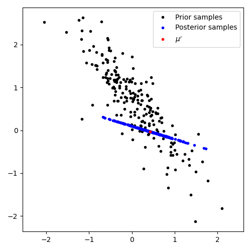
must hold for any possible \(A\). Thus we can remove all matrices from our prior which violate this equality constraint. This means we condition our multivariate Normal belief \(A \sim \mathcal{N}(A; \mu, \Sigma)\) on a subspace implied by the equality. Doing so is not a standard operation on multivariate Normals, but is possible and results in a rank-deficient multivariate Normal. The result is a new posterior belief \(A \sim \mathcal{N}(A; \mu', \Sigma')\).

Graphically, in 2D, this conditioning on a subspace looks as in this figure. (The detailed equation for conditioning a multivariate Normal on a subspace are in the appendix below.) The black dots are samples of possible matrices from the prior, and after conditioning on an observed subspace we retain a rank-deficient posterior, visualized by blue samples.

Thus, for our simple choice of multivariate Normal prior on \(A\) we can, for each observed \((z^{(m)}, y^{(m)})\) pair update our posterior beliefs analytically. (This update is relatively expensive and may preclude the Bayesian approach entirely, see discussion below.)

At any time, we can also compute the closed-form posterior over the trace itself, as it is a sum of Normal random variables and thus Bienayme's identity applies and moreover the resulting sum is again Normal. We have \(T \sim \mathcal{N}(\mu_T, \sigma^2_T)\), with

Overall this seems a satisfactory if computationally heavy model for trace estimation. But we can go further with the Bayesian approach and choose \(z^{(m)}\) intelligently using adaptive experimental design techniques.

Adaptive Experimental Design

Experimental design refers to making intelligent choices about what to measure in order to draw more informative inferences. In static experimental design one chooses a set of things to measure apriori, selecting measurements that for example are on average not too strongly correlated in order to maximize the expected information content of the measurements. The RQMC approach would be a simple example of a static experimental design because the \(z^{(m)}\) choices are dependent for different values of \(m\).

In adaptive experimental design we consider a sequential setting and thus sequentially decide what to measure based on all observations measured up to that point. You can think of adaptive experimental design as a simplification to the general reinforcement learning setup: your actions (what to measure) do not have an effect on the state of the world, and your reward is internal in terms of what information you have gained.

As a simple example, consider a paper survey setting: a static experimental design consists of a printed questionnaire with a set of well-chosen questions. An adaptive experimental design would only show one question to you at first and pick the next question based on your answer to all prior questions.

Personal anecdote. As a personal anecdote, I first used Bayesian experimental design to great effect in my work with Microsoft Israel on time-of-flight (ToF) camera technology (around 2013-2017). A time-of-flight camera is an active sensing system where time-modulated light is emitted into the world and the light bounces are recorded back on a camera, whose sensitivies are also time-modulated. By using Bayesian experimental design methods we were able to design the actively controllable part of the system and halve the mean absolute range estimation error (Section 7 in TPAMI 2016 paper) and to learn to measure maximally complementary information over time (dynamic time-of-flight CVPR 2017 paper). The Bayesian ToF approach shipped in a few thousand first-gen Hololens prototypes to developers but was replaced a year later with a different sensor and algorithm and unfortunately the entire Microsoft Israel time-of-flight team was let go, thus four years of hard work and my collaboration with an outstanding team in Israel, Amit Adam in particular, came to an end. (That is a separate story for another day.)

Later, in 2018, Cheng Zhang, Chao Ma, myself, and colleagues at Microsoft used adaptive Bayesian experimental design in more general settings such as questionnaire design (ICML 2019 paper, NeurIPS 2019 paper) and Cheng and team productized much of this work, now available through Azure and shipped in successful products.

For a wonderful introduction to experimental design and decision theory more generally, I highly recommend the book (Parmigiani and Inoue, "Decision Theory: Principles and Approaches", 2009).

For trace estimation, here is what the adaptive experimental design model would look like, visualized as influence diagram.

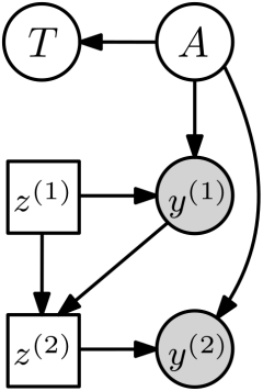
Choice nodes \(z^{(m)}\) are now rectangular to indicate that they are under our control and not independent random variables as before. How should we choose \(z^{(m)}\)? A natural approach is to select \(z^{(m)}\) as the one that maximizes the reduction in posterior uncertainty or variance. For this, denote all prior observations as \(\mathcal{D}_{<k} := \{(z^{(i)},y^{(i)})\}_{i < k}\). Then we can choose \(z^{(m)}\) as

This expression looks somewhat complex but here are some interpretation aids:

• It reads "variance before minus variance after". The "variance after", i.e. after additionally measuring \((z,y)\) is always smaller than the "variance before". Hence the objective measures the reduction in variance, which we want to maximize.
• The "variance after" term is also contained in an expectation over \((y,A)\). How come? We do not know \(y\) and \(A\), so we take an expectation over our best current beliefs up to that point.

The optimization problem may or may not have a closed-form solution, I did not investigate this. Instead, I did a simple implementation where I sample 100 points from \(\mathcal{N}(0,I)\), then pick the point that maximizes the objective.

Here is a small experiment. The experiment is smaller than small: with \(d=16\) I sampled \(A \sim \textrm{symmat}(\mathcal{N}_k(0,\Sigma_0)\), where \(k=d(d+1)/2\) and \(\Sigma_0\) is chosen such that \(\Sigma_{(i,i),(i,i)}=\sigma_d^2\) and \(\Sigma_{(i,i),(j,j)}=\sigma_o^2\) for \(i\neq j\). I used \(\sigma_d=200\) and \(\sigma_o=5\). This prior encodes diagonal-dominant matrices. To give the maximal possible edge to the Bayesian model I sampled \(A\) from this prior, i.e. there is no misspecification in this experiment. I ran 500 replicates of the trace estimation experiment, so the plots will be a bit noisy, but here are the results.

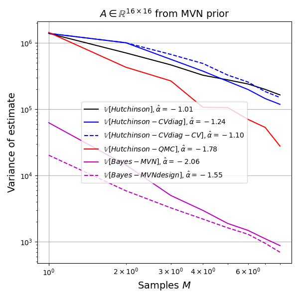
The Bayes model has an order of magnitude lower variance than the next best method (RQMC). The Bayesian method is not unbiased, so this low variance could be due to strong influence of the prior, so let's look at the root-mean-squared-error (RMSE) as well.

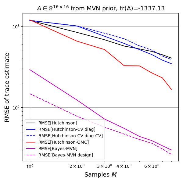
Again both Bayes methods are doing very well. If my implementation is correct, this must in fact be the case, as the Bayes estimate is optimal and thus the model achieves the Bayes risk in terms of RMSE. But is the model biased? The limited experiments do not allow a conclusion except that the plot shows that the unbiased methods show up as biased due to the estimated bias itself having an estimation error and the Bayesian models being in that same range.

Difficulties of the Bayesian approach

Clearly, the Bayesian approach to trace estimation is not ready to be used due to excessive runtime requirements. It may be possible to intelligently perform the same computation in terms of sparse updates or implicit representations of the evolution of \(\Sigma\), and thus make the Bayesian approach relevant.

Conclusion and Future Directions

We looked at a few existing estimators of the trace of a matrix. Here is a list of ideas for research in this area:

• Sequential or not? The estimators we have discussed can be divided into two classes. In the first class we have static estimators that can be parallelized because no computation depends on the output of prior computation. In the second class we have estimators that do some clever sequential processing (estimating control variates, estimating a low-rank approximation, or similar) and then benefit in a second stage. In practice, for deep learning applications, we may be able to get the best of both worlds by amortizing computation over time: instead of treating one optimization step as a closed-world, we can estimate the necessary quantities over multiple steps, for example in the control variate or low-rank approximation case. So the dichotomy between static and sequential is not as hard, which brings me to the following concrete idea.
• Parameterized control variates: in ML applications we often need trace estimates where the matrix \(A\) is a function of other quantities. For example, in diffusion models the matrix \(A\) may depend an input vector or time variable, e.g. \(A=A(x,t)\), and we do not have one trace estimation task but a large number of unique tasks with varying \(x\) and \(t\). This makes Hutchinson's estimator so popular: it is cheap in this setting, and this dependence on inputs seems to rule out approaches such as the control variate method which requires multiple samples. However, in reinforcement learning control variates called state-dependent baselines are commonly employed for variance reduction in policy gradient methods, e.g. (Tucker et al., 2018). So if our matrix has dependencies such as \(A(x,t)\) it may be beneficial to simultaneously learn a cheap control variate \(B(x,t)\), perhaps as an auxiliary output of the main model, in order to amortize computation over learning iterations, in effect is a simple form of learning-to-learn more efficiently.
• Bayesian trace estimation? Conceptually the Bayesian approach is particularly attractive for trace estimation as the latent structure of the problem is exactly known. In practice I have my doubts whether this approach will be useful in deep learning, for three reasons: 1. already the simplest faithful model I could come up with is computationally very expensive; 2. it seems challenging to find suitable priors \(p(A)\) over matrices for two reasons, a) standard choices such as Wishart distributions are not closed under subspace conditioning so must be handled using even more expensive computational approaches, and b) trace estimation is used in a wide variety of domains and a generally useful yet uninformative prior seems too much to ask for; and 3. unbiasedness is highly desirable in most deep learning uses of trace estimation and Bayesian estimates are generally biased in the small sample setting and only asymptotically unbiased for \(M \to \infty\), whereas Hutchinson's estimator is unbiased for any \(M\). Finding a general prior for matrices that is computationally efficient under subspace conditioning would could be interesting. Perhaps a good starting point would be the multivariate Normal distribution but then to marginalize most dimensions away. This would make computation more efficient while retaining tractability.

So there you have it. Given my understanding so far, I even venture to make some recommendations for the current estimators:

1. First, use Hutchinson's estimator or the Gaussian trace estimator. Try both and measure the variance.
2. If you can afford \(M > 1\) and \(d < 21,201\): give the RQMC approach a try; it should be simple to implement, with SciPy, Tensorflow, and PyTorch all supporting Sobol sequence generation. (The restriction to \(d < 21,201\) is not intrinsic to the approach but a practical constraint due to limited availability of so called direction numbers.)
3. If variance of the estimates in your trace estimates are a major bottleneck in your application, try the diagonal control variate approach, perhaps learning this control variate as part of your learning objective if the matrix is varying with the inputs to your network.

Acknowledgements. I thank Yang Song for careful reading and feedback on the draft including a number of corrections and pointing me to two more uses of trace estimation; to Florian Wenzel for corrections, references, and improvements to the quasi Monte Carlo methods.

Appendix

Conditioning a multivariate Normal on a subspace

First, the following result: if \(x \sim \mathcal{N}(\mu,\Sigma)\), and

then \(T(x) \sim \mathcal{N}(A\mu + b, A\Sigma A^T)\). Furthermore we have joint Normality,

Observing \(y=T(x)\) we have \(x | y \sim \mathcal{N}(\bar{\mu},\bar{\Sigma})\), with