How good are your beliefs? Part 1: Scoring Rules
Posted on Fri 04 September 2015 in Statistics, Machine Learning
This article is the first of two on proper scoring rules, a specific type of loss function defined on probability distributions or functions of probability distributions.
If this article sparks your interest, I recommend the gentle introduction to scoring rules in the context of decision theory in Chapter 10 of Parmigiani and Inoue's "Decision Theory" book, which is a great book to have on your data science bookshelf in any case and it deservedly won the DeGroot prize in 2009.
Scoring Rules
Consider the following forecasting setting. Given a set of possible outcomes \(\mathcal{X}\) and a class of probability measures \(\mathcal{P}\) defined on a suitably constructed \(\sigma\)-algebra, we consider a forecaster which makes a forecast in the form of a probability distribution \(P \in \mathcal{P}\). After the forecast is fixed, a realization \(x \in \mathcal{X}\) is revealed and we would like to assess quality of the prediction made by the forecaster.
A scoring rule is a function \(S\) such that \(S(P,x)\) is taken to mean the quality of the forecast. Hence the function has the form \(S: \mathcal{P} \times \mathcal{X} \to \mathbb{R} \cup \{-\infty,\infty\}\). There are two variants popular in the literature: the positively-orientied scoring rules assign higher values to better forecasts, the negatively-oriented scoring rules behave like loss functions, taking smaller values for better forecasts.
A proper scoring rule has desirable behaviour, to be made precise shortly. Let us first think what could be desirable in a scoring rule. Intuitively we would like to make "cheating" difficult, that is, if we really subjectively believe in \(P\), we should have no incentive to report any deviation from \(P\) in order to achieve a better score. Formally, we first define the expected score under distribution \(Q\),
So that if we believe in any prediction \(P \in \mathcal{P}\), then we should demand that (for negatively-oriented scores)
For strictly proper scoring rules the above inequality holds strictly except for \(Q=P\). For a proper scoring rule the above inequality means that in expectation the lowest possible score can be achieved by faithfully reporting our true beliefs. Therefore, a rational forecaster who aims to minimize expected score (loss) is going to report his beliefs.
Key uses of scoring rules are:
- Evaluating the predictive performance of a model;
- Eliciting probabilities;
- Using them for parameter estimation.
Let us look briefly at the different uses.
Model Evaluation
For assessing the model performance, we simply use the scoring rule as a loss function and measure the predictive performance on a holdout data set.
Probability Elicitation
For probability elicitation we can use a scoring rule as follows: we ask a user to make predictions and we tell him that we will reward him proportionally to the value achieved by the scoring rule once the prediction can be scored. Assuming that the user is rational and aims to maximize his reward, if we use a proper scoring rule, then he can maximize his expected reward by making predictions according to the true beliefs he holds. However, while the existence of a strictly proper scoring rule roughly means that elicitation of a quantity is possible, more efficient methods for probability elicitation may exist. Infact, Simon French and David Rios Insua argue in their book Statistical Decision Theory, page 76, that
"de Finetti (1974; 1975) and others have championed the use of scoring rules to elicit probabilities of events. ... Scoring rules are important in de Finetti's development of subjective probability, but it is not clear that they have a practical use in statistical or decision analysis. ... Scoring rules could provide a very expensive method of eliciting probabilities. In training probability assessors, however, they can have a practical use."
If you wonder what more efficient alternatives French and Insua have in mind, they do propose several methods to elicit probabilities, such as an idealized "probability wheel" the user can configure and spin, and a sequence of proposed gambles in order to find a fair value accepted by the user.
In general it seems to me (as an outsider of this field), that probability elicitation is as much about theoretically sound methods as it is about human psychology and biases, and how to avoid them. The human aspect of probability elicitation is discussed in the Roger Cooke's book-length monograph on the topic, and the recent study of (Goldstein and Rothschild, "Lay understanding of probability distributions", 2014) (thanks to Ian Kash for pointing me to this study!).
Estimation
For parameter estimation we perform empirical risk minimization on a probabilistic model using the scoring rule as a loss function, an approach dating back to (Pfanzagl, 1969). This is a special case of M-estimation but generalizes maximum likelihood estimation (MLE), where the log-probability scoring rule is used.
If the model class contains the true generating model this yields a consistent estimator but for misspecified models this can yield answers different from the MLE, and these answers may be preferable; for example, if model assumptions are violated and for any choice of parameter the model would put have a low density on some observations these tend to influence the MLE severely because the log-prob scoring rule assigns a large penalty to these observations. Using a suitable scoring rule cannot prevent misspecification of course but the consequences can be made less severe.
It should also be said that for estimation problems the log-prob scoring rule is the most principled in that it is the only one that can be justified from the likelihood principle.
Scoring Rule Examples
Here are a few examples of common and not so common scoring rules both for discrete and continuous outcomes.
Scoring Rule Example: Brier Score
This scoring rule was historically the first, proposed by Glenn Wilson Brier (1913-1998) in his seminal work (Brier, "Verification of Forecasts Expressed in Terms of Probability", 1950) as a means to verify weather forecasts.
Given a discrete outcome set \(\{1,2,\dots,K\}\) the forecaster specifies a distribution \(P=(p_1,\dots,p_K)\) with \(p_i \geq 0\) and \(\sum_i p_i = 1\). Then, when an outcome \(j\) is realized we score the forecaster according to the Brier score,
The Brier score is extensively discussed in (DeGroot and Fienberg, 1983) and they show that it can be decomposed into two terms measuring calibration and refinement, respectively. Here, refinement measures the information available to discriminate between different outcomes that is contained in the prediction.
For the case with binary classes, the definite work is (Buja, Stuetzle, Shen, 2005) in which a class of scoring rules is proposed based on the Beta distribution which generalizes both the Brier score and the log-probability score.
Scoring Rule Example: Log-Probability
The most common scoring rule in estimation problems is the log-probability, also known as the log-loss in machine learning. Maximum likelihood estimation can be seen as optimizing the log-probability scoring rule.
For the discrete outcome case it is given simply by
If \(p_i = 0\) the score \(S_{\textrm{log}}(P,i) = \infty\). The log-probability is a proper scoring rule, but what really distinguishes it is that it is local in that when outcome \(j\) realizes only the predicted value \(p_j\) is used to compute the score. Intuitively this is a desirable property because if \(j\) happens, why should we care about the precise distribution of probability mass for the other events?
It turns out that this local property is unique to the log-probability scoring rule. (For the result and proof see Theorem 10.1 in Parmigiani and Inoue's book.)
Scoring Rule Example: Energy Statistic
This scoring rule is for predicting a distribution in \(\mathbb{R}^d\) and is defined for \(\beta \in (0,2)\), realization \(x \in \mathbb{R}^d\), and distribution \(P\) on \(\mathbb{R}^d\) as
This score has an intuitive interpretation: the score is the expected distance to the realization minus half the expected pairwise sample distance. Let us think about a few cases: if \(P\) is a point mass, then the first term is just the distance to the realization and the second term is zero; in particular for \(\beta \to 2\) the score recovers the squared Euclidean norm loss. The original definition is from (Gneiting and Raftery, 2007) except for the sign change, but is based on Szekely's energy statistic which also independently found its way into machine learning through the Hilbert-Schmidt independence criterion.
For \(\beta \in (0,2)\) the energy score is a strictly proper scoring function for all Borel measures with finite moment \(\mathbb{E}_P[\|X\|^\beta] < \infty\).
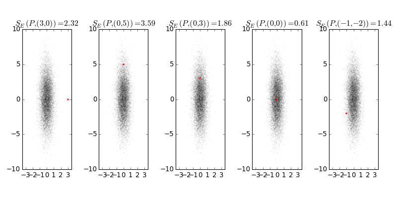
Here is a visualization, where \(P = \mathcal{N}([0,0]^T, \textrm{diag}([1/2, 5/2]))\) is given by the 10k samples and the red marker corresponds to the realization \(x\). Here we have \(\beta=1\). We can see that the Euclidean nature of the scoring rule seems to dominate the anisotropic distribution \(P\), that is, a realization that is unlikely under our belief distribution (leftmost plot) achieves a lower score than a sample with higher density (second leftmost plot).
As a practical manner, the energy score is simple to evaluate even when you have only predictive Monte Carlo realizations of your model, compared to the log-probability rule which requires the normalizer of the predictive distribution.
Scoring Rule: Check Loss
The check loss, also known as quantile loss or tick loss, is a loss function used for quantile regression, where we would like to learn a model that directly predicts a quantile of a distribution, but we are given only samples of the distribution at training time.
This scoring rule is somewhat different in that a specific property of a belief distribution is scored, namely the quantile of the distribution. Being proper here means that the lowest expected loss is achieved by predicting the corresponding quantile of your belief. (Interestingly proper scoring rules exist only for some functions of the distribution, see (Gneiting, 2009).)
You may know a special case of the check loss already: when using an absolute value loss, your expected risk is minimized by taking the median of your belief distribution, that is, the \(\frac{1}{2}\)-quantile. The check loss generalizes this to a richer family of loss functions such that the expected minimizer corresponds to arbitrary quantiles, not just the median. Thus, instead of scoring an entire belief distribution \(P\) we only score its quantile statistics.
The check loss is defined as
where \(r\) is our predicted \(\alpha\)-quantile and \(x \sim Q\) is a sample from the true unknown distribution \(Q\).
Plotting this loss explains the name check loss and tick loss, because it looks like two tilted lines. I show it for a sample realization of \(x=5\), and the horizontal axis denotes the quantile estimate.

For any belief distribution, taking the minimum expected risk decision yields the matching quantile. For example, if your beliefs are distributed according to \(X \sim N(5,1)\), then you would consider the expected risk
This convolves the check loss function with the belief distribution, in this case corresponding to a Gaussian kernel. The minimizer over \(r\) of this expected risk function would correspond to your optimal decision.

The above plot marks the 10/50/90 quantiles and these correspond to the minimizers of the expected risks of the respective check losses.
Conclusion
The above is only a small peek into the vast literature on scoring rules. If you are mathematically inclined, I highly recommend (Gneiting and Raftery, 2007) as an enjoyable further read and (Frongillo and Kash, 2015) for the most recent general results; everyone else may enjoy the book mentioned in the introduction.
In the second part we are going to put your forecasting skills to the test via an interactive quiz!
Acknowledgements. I thank Ian Kash for further insightful discussions on scoring rules and pointing me to relevant literature.