Extended Formulations
Posted on Sun 05 April 2015 in Optimization
An amazing fact in high dimensions is this: Projecting a simple convex set described by a small number of inequalities can create complicated convex set with an exponential number of inequalities.
It is amazing because it contradicts our everyday human experience. We are most familiar with projections of objects in three dimensions down to two dimensions, namely when objects cast shadows, like this:
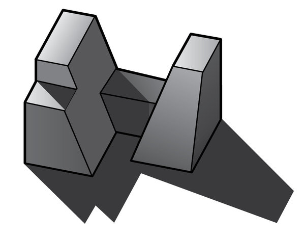 (Image courtesy to Cloud Nines
Designs.)
(Image courtesy to Cloud Nines
Designs.)
In three dimensions any polyhedral object, when projected onto a plane, becomes simpler, i.e. the number of facets stays the same or becomes smaller. Think of a three dimensional cube that casts a shadow. The cube has six facets but its shadow has four or six, depending on the position of the light and plane. [Edit and correction, July 2015: Thanks to reader Paul (comment below), I have been made aware that it is not true that the number of facets cannot increase when projecting form three dimensions onto the plane. A great example is provided by Sebastian Pokutta, where a convex 3D polytope with six facets projects onto the 2D plane as an octagon with eight facets. Thanks Paul!]
Now, how I can I convince you that a convex set can become more complex when projected? Here is an impressive example.
Ben-Tal/Nemirovski Polyhedron
The following example is from (Ben-Tal, Nemirovski, 2001), (PDF). In this paper the authors are motivated by approximating certain second order cones using extended polyhedral formulations, in order to be able to perform robust optimization using linear programming. As a special case of their results I select the problem of approximating a unit disk in the 2D plane. (The following is a specialization of equation (8) in the paper.)
First, let us fix some notation. Let \(x=(x_1,x_2,\dots,x_n,\alpha_1,\dots,\alpha_m) \in \mathbb{R}^{n+m}\) be a vector, where \(x_1\) to \(x_n\) represent the basic dimensions and \(\alpha_1\) to \(\alpha_m\) represent the extended dimensions. For any set \(\mathcal{E} \subseteq \mathbb{R}^{n+m}\) we define the projection as
This corresponds to the familiar notion of a projection.
For the 2D unit disk the following is an extended polyhedral formulation, parametrized by an integer accuracy parameter \(k \geq 2\). The formulation has the basic dimensions \(x_1\) and \(x_2\), and the extended dimensions \(\mathbf{\alpha}=(\xi_j,\eta_j)_{j=0,\dots,k}\). Defining the constants \(c_j = \cos(\pi / 2^{j})\), \(s_j = \sin(\pi / 2^j)\), and \(t_j = \tan(\pi / 2^j)\) the polyhedral set \(\mathcal{E}_k\) is given by the following intersection of linear inequality and equality constraints.
Note that the set \(\mathcal{E}_k\) can be described by \(6+3k\) sparse linear constraints. The intersection of these convex constraint sets is of course again a convex set. Thus, the description of the set takes \(O(k)\) space, where \(k\) is the approximation parameter.
If we write \(\mathcal{D}_k := \textrm{proj}_{x_1,x_2} \mathcal{E}_k\) for the projection onto the first two dimensions, the following figure illustrates just how remarkably accurate the formulation is as we increase \(k\).

How accurate is it? Ben-Tal and Nemirovski say that a set \(\mathcal{D}\) is an \(\epsilon\)-approximation to a set \(\mathcal{L}\) if \(\mathcal{L} \subseteq \mathcal{D}\) and if for all \(x \in \mathcal{D}\) it holds that \((\frac{1}{1+\epsilon} x) \in \mathcal{L}\). They then show that the above formulation is an \(\epsilon_k\)-approximation, where
That is, despite having a compact description in \(O(k)\) space the accuracy improves exponentially. In the basic dimensions the set \(\mathcal{D}_k\) has exponentially many facets and cannot be described compactly through a polynomial sized collection of linear inequalities. (The paper further generalizes the above results to the family of \(d\)-dimensional Lorentz cones.)
Is there a Recurring Pattern?
The abstract idea behind obtaining complicated structures in one space by means of something like an extended formulation can be found in other domains; for example, in probabilistic graphical models.
Suppose we would like to specify a potentially complicated probability distribution \(P(X)\). Akin to an extended formulation we may proceed as follows. We define an extended set of random variables \(\alpha\) and a distribution \(P(\alpha)\). We then couple both spaces by means of a conditional specification, \(P(X|\alpha) P(\alpha)\). We then project, that is, marginalize out, the extended dimensions \(\alpha\) to obtain
In practice this construction is often used in the form of a hierarchical graphical model, for example when using a Normal mixture to define a student T distribution.
The increase in flexibility of the resulting marginal distribution can be as impressive as for the above polyhedral sets: for example, if \(P(X|\alpha)\) is a Normal distribution and \(P(\alpha)\) is a distribution over Normal parameters, then the infinite Normal mixture can essentially represent any absolutely continuous distribution.
Another observation, which may be just a coincidence, but maybe there is more to it: the extended formulation construction in both cases suggests a practical implementation. In the polyhedral set this was through linear programming in the extended space, for the graphical model it would be ancestral sampling or MCMC inference.
This leaves me with the following questions:
- Are there more examples of similar constructions (extension, coupling, projection)?
- What is the shared mathematical structure behind this similarity (e.g. permitting a projection operation that leads to complexity in the basic dimensions that no longer admits a compact description in this space)?
Feedback very much welcome :-)
Conclusion
I first learned of extended formulations from this book of Pochet and Wolsey, who pioneered the technique for practical scheduling optimization problems. (Yes, I had enough time for tinkering during my PhD to take such creative diversions.) A recent summary of extended formulations for combinatorial optimization problems is Conforti, Cornuejols, Zambelli, 2012.
Many so called higher-order interactions in computer vision random field models are representable as extended formulations, a point I elaborated on in a talk I gave at the Inference in Graphical Models with Structured Potentials workshop at the CVPR 2011 conference. Another relevant work is Miller and Wolsey, 2003.